Continuing Education

I’ve recently become interested in machine learning and have been studying it in my spare time. My motivation is AI safety. A superhuman artificial intelligence has the potential for a tremendously positive or tremendously negative impact on an enormous number of lives. Therefore, it’s crucial that if we develop one, we do so safely. Many resources are being poured into advancing AI’s capabilities, but only a tiny amount are being spent on solving safety problems.

I’m learning about this field in the hope that I can contribute one day. To begin building up my knowledge, I’ve been taking self-directed online courses.

Google ML Crash Course

The first course I took was the Machine Learning Crash Course from Google. Before I started, I considered myself a complete novice when it came to ML. However, I discovered that I was already familiar with many of the concepts, such as gradient descent and overfitting. ML may use different jargon, but it shares a lot with traditional disciplines.

I appreciated the fact that when the course introduced a technique, they gave a brief comparison to alternatives we’d already seen, along with some rules of thumb about which to use when. Knowing how something works is important, but so is knowing when to use it.

The time I found this most useful was in learning about regularization, which is a set of techniques to reduce overfitting. The motivation for regularization was clear to me, but I wasn’t familiar with the specifics. The course explained that L₁ regularization, which aims to minimize the absolute values of a model’s weights, can drive some weights to zero, which helps to improve computational performance when there are a large number of features (inputs). L₂ regularization, which aims to minimize the square of the weights, will tend to keep weights from getting too large. But it typically doesn’t drive them to exactly 0 because its effect on the gradient diminishes as the weights get smaller. Dropout regularization, which removes random nodes from the network at each iteration, is similar to averaging over an ensemble of smaller networks.

fast.ai Practical Deep Learning for Coders

The creators of fast.ai, which supplements the popular PyTorch library, offer their own introductory machine learning course. While I was in the middle of the course, they released an updated 2022 version. My comments here are about the earlier 2020 version, so I apologize if any of them are out of date.

For me, one key takeaway from the course was the importance of picking a good baseline to compare a ML model to. An accuracy of 75% may sound good, but if always picking the average would give an accuracy of 80%, it’s clear the ML model isn’t performing well. However, a trivial baseline isn’t always the best choice. Sometimes it’s better to use a heuristic that is much simpler than the ML model but still captures some of the underlying relationship. Ultimately, just as one would make a best effort on developing a ML model, one should make a best effort on a non-ML baseline.

The course devoted one of its eight lectures entirely to ethics discussions, a substantial amount for an introductory course like this. The lecturer for that class, Rachel Thomas, shared many examples of the negative effects ML and AI can have, with some questions to keep in mind to help catch potential problems early. While there usually aren’t clear solutions to these sorts of ethical issues, at least being aware of how many ways things can go wrong reinforces the point that everyone in the field should feel responsible for thinking about and working on them.

Dr. Thomas made the explicit point to focus on ethical issues of the present that are affecting people now and not on issues that future generations may face. Six months ago, I would have whole-heartedly agreed. Why spend time on hypothetical future problems when we have concrete ones in front of us today?

However, I’ve recently changed my mind about this. Some problems may not be possible to solve once they are realized. For instance, it might be impossible to switch off a superhuman AI if it starts acting in undesirable ways. Therefore some problems need to be prevented altogether and not addressed reactively.

It’s also important to keep in mind that the future will likely have many more people than the present, not just at any moment but especially in total. And their concerns are particularly neglected today: they can’t vote, protest or advocate for themselves. To me, that’s all the more reasons to prioritize the issues of the future, like figuring out how to create an AI that aligns with our values, now.

NYU Deep Learning

The third ML course I took was NYU’s Deep Learning with Professor Yann LeCun, which was much more substantial than the previous two courses I took. I followed the material from the 2021 version of the course , which was the most recent one available at the time. The lectures were split between LeCunn and assistant professor Alfredo Canziani, whom I have to thank for making this material freely available. I enjoyed Canziani’s teaching style, visualizations and attention to detail in the slides. The 2021 version of the course placed a big emphasis on energy-based models, which weren’t a concept I had come across before, at least not formally.

My overall biggest criticism of the course is that the lectures had little relevance to the later assignments. While the first two courses I took held my hand a little too much, this one was quite the opposite. I had to do a lot of self-teaching to complete the assignments. While I perhaps ended up learning the material more thoroughly, this made progress slow.

Recurrent Neural Network (Notebook)

One of the assignments used a recurrent neural network to echo back the input string delayed by a variable amount: for instance delaying abcdef by three should yield XXXabc, where X is a placeholder indicating a lack of output. The dataset for this assignment consisted of random strings of 20 characters with random delays between 0 and 8 (inclusive). The instructions were to train a model to achieve a particular accuracy within a limited amount of training time.

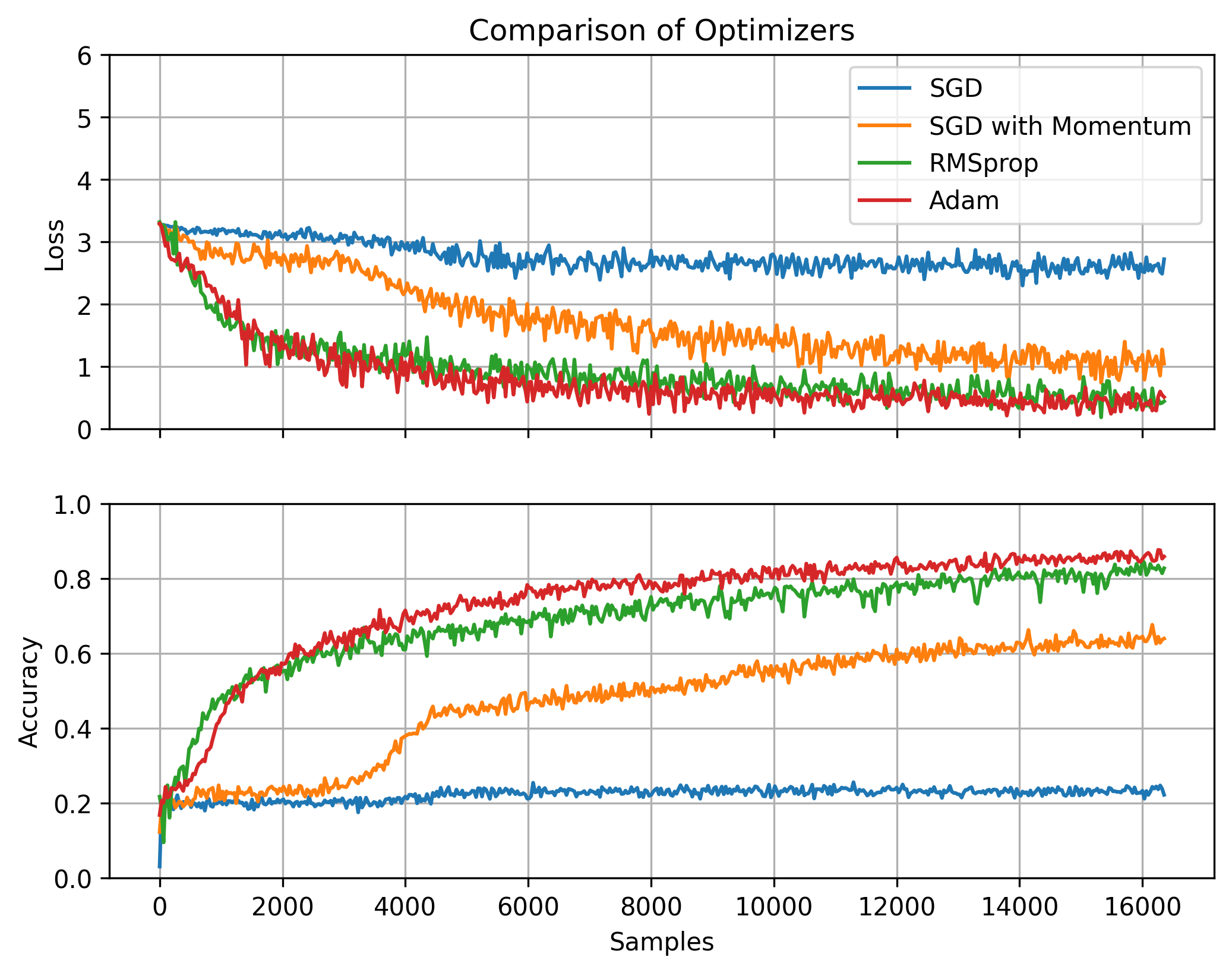
Reaching the desired accuracy within the time limit wasn’t especially challenging. But it made me curious about how different factors affected the training speed. I experimented with different optimizers and batch sizes. Of course there are plenty of other factors that might have an impact, but I decided to focus on these and found some unexpected results.

Optimizer

I was surprised how much of a difference the choice of optimizer made. For each one, I experimented with a range of different hyperparameter values to find the best ones. Default SGD performed very poorly. Introducing some momentum noticeably improved the training rate. But the RMSprop and Adam optimizers were better still. Results in the following section were obtained with Adam.

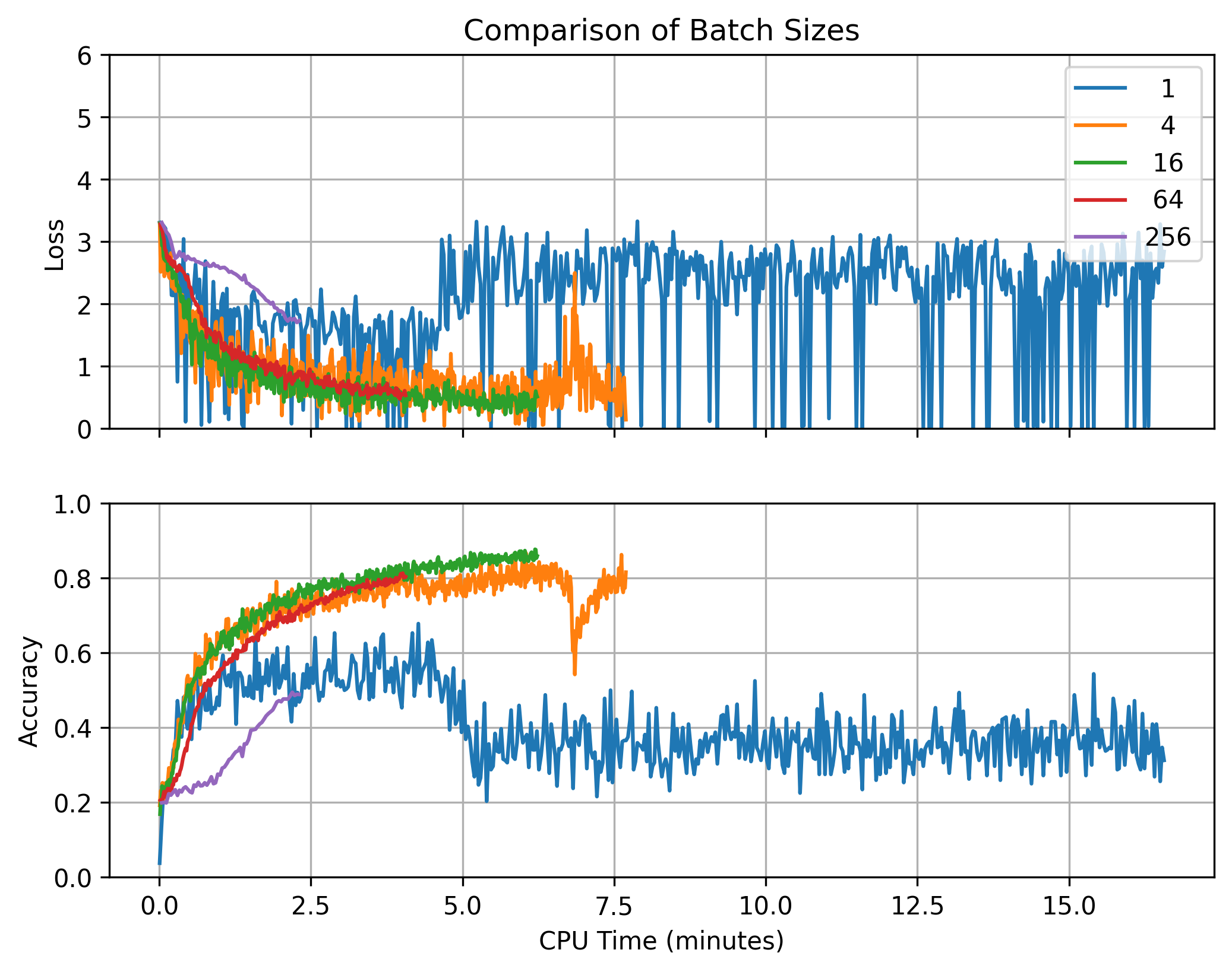
Batch Size

The effects of batch size were more expected. For small batch sizes, progress was noisy since each step was based on a smaller number of samples. But as the batch size got large, training slowed down since the extra samples per step weren’t adding much information.

Larger batches allowed the model to more quickly consume the training set (2¹⁴ = 16,384 samples for these experiments). In part, this was because the calculations could be run in parallel on different CPU cores. But time continued to decrease even as the batch size exceeded the number of cores. This can be explained by the fact that the optimizer took fewer steps, meaning it spent less time backpropagating gradients and updating parameters.

Convolutional Neural Network (Notebook)

Another assignment used a convolutional neural network (CNN) to convert images to text, taking an energy-based approach to dividing the image into individual characters. The dataset for this assignment was generated on demand using Python’s Pillow library to convert strings to small images. This is admittedly much simpler than using handwritten text and also has the advantage of offering unlimited training examples.

A CNN operates by sliding a window across the image, examining only a portion of the pixels at a time. When the window lines up with a letter, like the a in the example below, the logit associated with that letter ideally lights up. Sometimes the window straddles two characters. Other times it’s located over blank space near the edges of the image. In these situations, it’s helpful for the model to know it’s not looking at exactly one character and output a _ placeholder token instead. To train this behavior, the characters of each input string were separated by this placeholder: abc became a_b_c_.

Single character recognition is a simple classification problem: if the image is of a letter a, adjust the weights to increase the confidence that the model predicts a. For multicharcter strings, one might naively generalize this to boosting the a logit whenever there’s an a in the image. But this doesn’t give the model any information about where the a is. For text recognition, the order of the characters matters as much as the characters themselves. The naive strategy would give the model the exact same update for ab as it would for ba, meaning the model would never learn to predict the order of the characters.

One can train much more effectively by targeting the weights that contribute to the a prediction at a particular location within the image. For a fixed-width font like the one used in this assignment, one could say that the first W pixels contain the first character, and the second W pixels contain the second character. But this requires all characters to have the same known size and doesn’t generalize to other scenarios. In essence, a model trained this way would only be able to recognize single characters and would rely on the input being split up correctly.

Instead, it would be better to have the model divide up the image itself. To train it to do so, the model logits were calculated for each character in the input and each window location within the image. This created a heat map like the one below, with character class on the vertical axis and window location on the horizontal axis. A point in this heat map is a measure of how strongly the model thinks the given area in the image contains the given character. Typically, the higher the logit value, the higher the probability. But in this case, the logits were interpreted as energies, where lower is better.

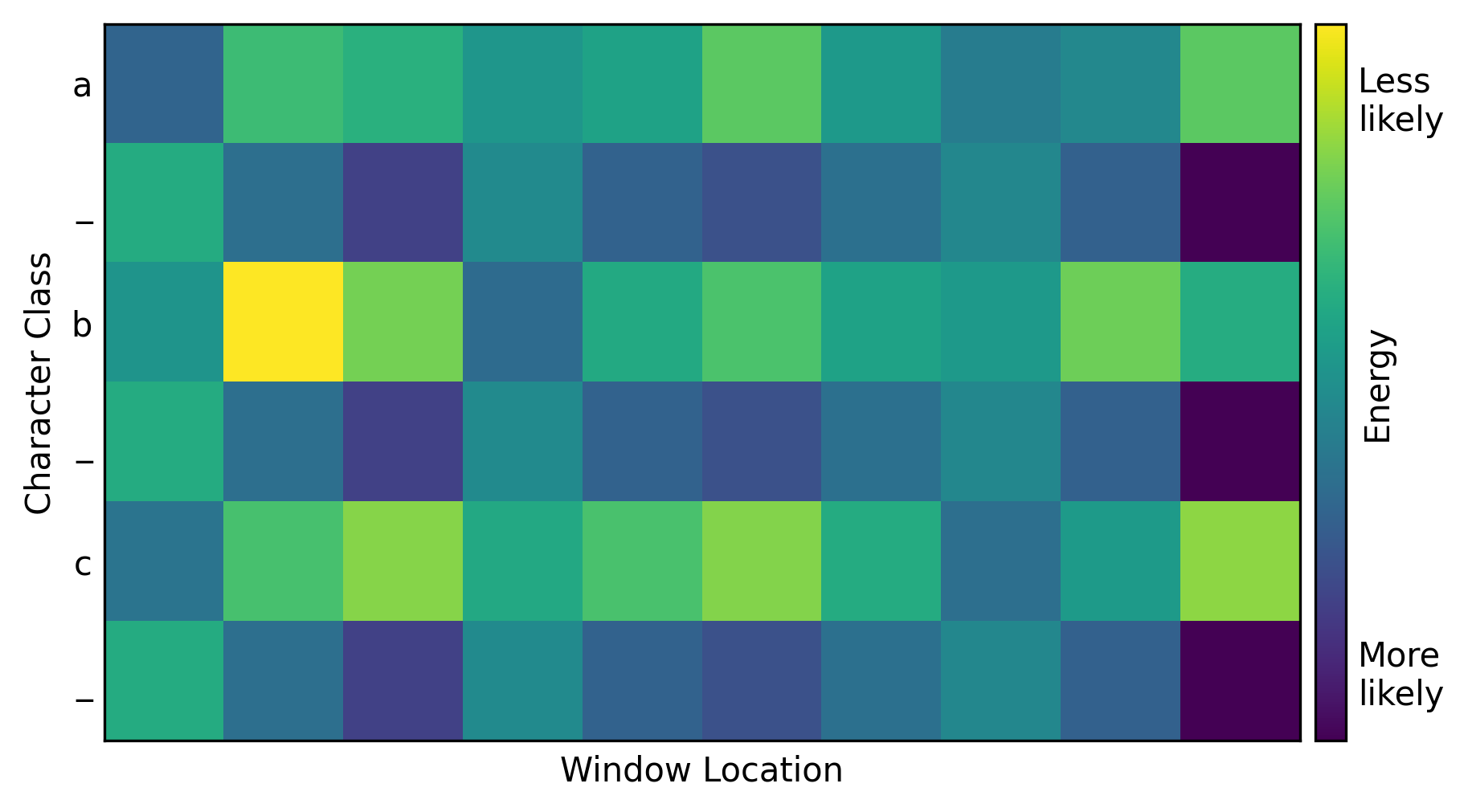
The top left corner indicates the model’s measure of whether the first window location contains the first character. Immediately to the right is the measure of whether the second window location contains the first character, and so on across the top row. The second row contains the predictions for the second character at each window location.

One can use this heat map to determine how the model has divided up the image into characters. A mapping from window location to character can be thought of as a path through the heat map. A valid path must begin in the upper-left corner since the left side of the image corresponds to the beginning of the string. Similarly, the path must end in the lower-right corner since the right side of the image corresponds to the end of the string. Between these two corners, a valid path must move monotonically down and to the right without skipping any rows or columns. The best way to divide the image, according to the model, is the path with least total energy. This can be found with a search algorithm such as Djikstra’s or even brute-force since the number of valid paths is small for heat maps of this size.

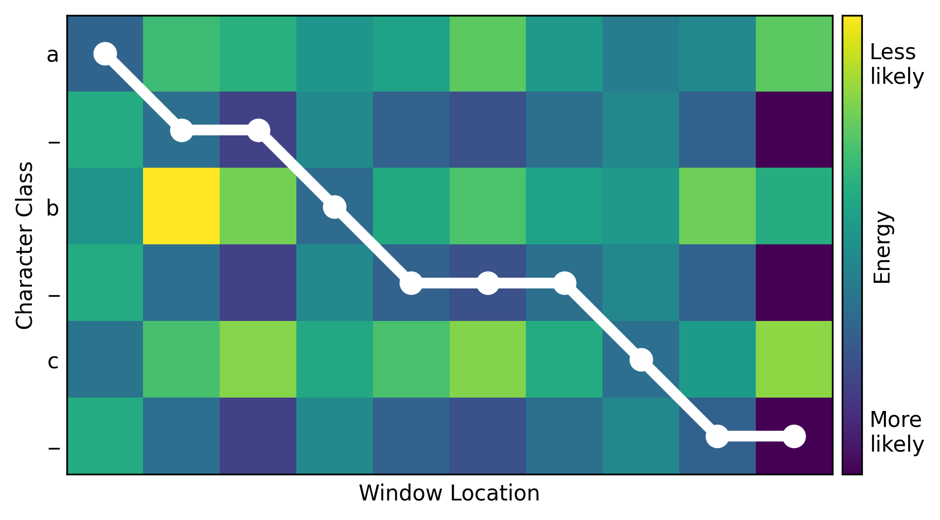
Adding up the energies along the optimal path produced the total loss. Minimizing this loss efficiently trained the model to improve its predictions at the relevant locations within the image.

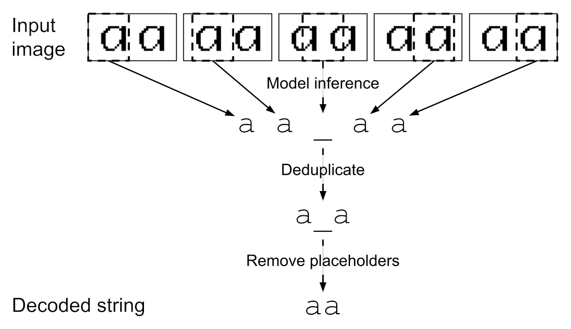
At inference time, the model’s prediction was determined by applying the argmin function (remember: lower energy is better) across the 27 character classes at each window location within the image. Duplicates were common since the window size could be larger than a character, so they were dropped to avoid counting the same character multiple times in a row. Because the model was trained to to predict a placeholder _ between actual letters, legitimate repeats were preserved.

The model achieved an accuracy of over 90% after training on two character strings for 30,000 samples. However, this wasn’t enough for it to generalize from two characters to more. For three characters, the accuracy was 0%. Further training on longer strings strongly improved its accuracy at decoding them.